Introduction

Understanding algorithms and data structures is a key pillar in computer science. Developers are problem solvers and often times it is not about how to solve a problem, but how to efficiently solve it.

There are a variety of problems that can be solved using algorithms related to sorting, searching, graphing, strings, and so much more.

How we measure the performance of an algorithm? What metrics can be used to determine if an algorithm is sufficient for a given problem? That is where the Big-O notation comes into play.

Simply put, Big-O notation is a useful mathematical notation that is used to determine algorithmic complexity. It determines performance in the worst-case scenario and provides an upper boundary on the growth rate of an algorithm in relation to the input.

For example, say you are searching for an item in an array of n items one by-on. The worst-case scenario is searching all n items to find the match. In this case, we say the performance of such an algorithm is O(n).

There are different terminologies used to describe common algorithmic complexities such as constant time, linear time, quadratic time, logarithmic time, and so much more. We will explore these in great detail as we cover Big-O notation.

Big-O Notation

When you learned about polynomials in school, you learned about terms and more specifically, dominant terms. When it comes to describing scalability, we omit the lesser terms and focus on the dominant term of a given polynomial.

That is because the size of the dominant term is what makes the greatest impact on the value of the polynomial.

For instance, consider the quadratic polynomial in the following form:

ax² + bx + c

The dominant term will always be ax² because as the input size grows, the output is greatly impacted by the ax² term. The constant value, c always remains the same and bx is always a linear term and so it grows linearly.

We can assume that for significantly large input values, the linear and constant terms will not affect the output to the extent the quadratic term would so we can simplify to ax² or in Big-O notation terminology, O(ax²).

Since a is also a constant associated with the quadratic term, we can further simplify this and state that the quadratic polynomial has a complexity of O(x²).

In the study of algorithms, this complexity is known as quadratic time. When analyzing algorithms, we can describe code as a sum of algebraic terms.

We can deduce the dominant term and therefore determine its runtime complexity using Big-O notation.

Code Overview

You might be wondering how we determine what terms to use to describe runtime complexity. We will explore that in this section.

You can clone the following repository. The directory of concern is demos/Demo38_Polynomial_Time_Big_O_Notation.

In this directory, you will find the polynomialTime.ts file containing the following code:

Loading GitHub Gist...

Constant time refers to lines of code that accomplish a single task. No matter how many times you iterate through the code, you will always run through it once.

For loops, we can assume that we iterate over it n times (if it is an array of length n, it is n times). Runtime complexities for loops is linear time or O(n).

Nested loops are interesting. Since we are running a loop within a loop, we can assume that iterations and sub-iterations will be of the n x n order or O(n²), quadratic time.

The higher the number of nested loops, the higher the degree of growth and runtime complexity [3 loops O(n³), 4 loops O(n⁴), … , m loops O(n^m)].

In the codebase above, you can see highlighted sections referring to constant, linear, and quadratic times.

Calculating Runtime Complexity

When studying algorithms, the most efficient ones scale based on input size. This is important because computations involving inefficient algorithms can be expensive in terms compute resources and time.

Analyzing performance in the worst-case scenario is what drives efficiency because it determines the effectiveness of an algorithm in extreme cases.

The following chart illustrates common runtime complexities pertaining to algorithms:

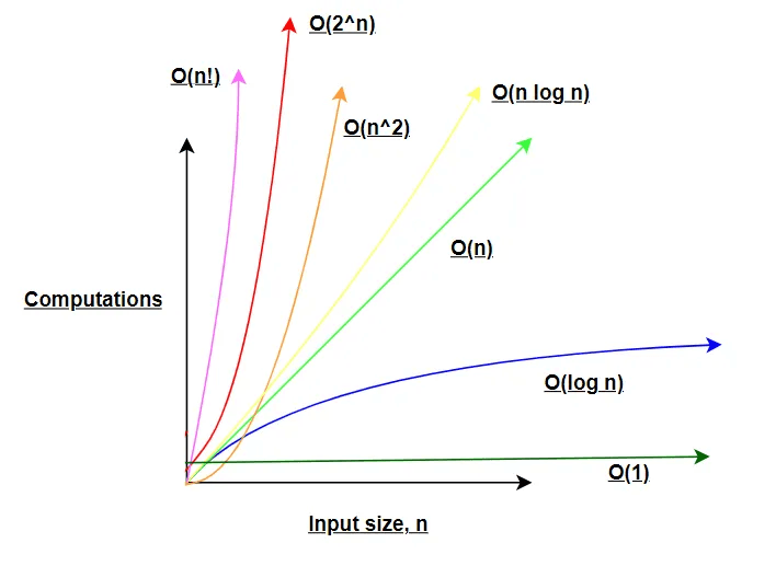
As the input size increases, the order of growth is an important consideration.

We have looked at constant time O(1), linear time O(n), and quadratic time O(n²).

The worst-time complexity is factorial time O(n!), followed by exponential time O(2^n), and so on. Algorithms that scale in linear O(n), linearithmic O(n log n) or logarithmic time O(log n) are preferred.

In a perfect world, we would like to see a runtime complexity of constant time O(1), but that is not possible.

In the example above, we make use of the popular binary search algorithm to efficiently search for an item in an ordered array. The algorithm scales efficiently because it uses what is known as partitions to numerically separate sections of the array where the value might be located.

Partitions are created in pairs and further ones are created until a search is found. For instance, say you are searching for number 6 in an ordered array of 10 items, the first partition would separate the array into 1–5 and 6–10.

After that, we check to see if the value is greater than or less than the value in the middle (input size/2) to determine which partition to search next.

In this case, 6 is greater than 5 so we search the second partition following the same process until 6 is found.

This algorithm has a logarithmic runtime complexity, O(log n) and scales efficiently for any input size.

Searching each item in the array one by one would be feasible as well, but that would yield a linear runtime complexity, O(n).

The binary search algorithm yields a more efficient solution to the search problem and is just one example of many where algorithms provide efficiency.

Now we can calculate the runtime complexity of the entire application using simple algebraic terms. The section where constant time is discussed can be represented with an integer.

The section discussing linear time has a runtime complexity of O(n). The section discussing quadratic time has a runtime complexity of O(n²).

Finally, the section discussing the binary search algorithm (as noted earlier) has a runtime complexity of O(log n).

The sum of all these can be represented with the following:

n² + n + log(n) + 1

Since the most dominant term is n², it follows that the runtime complexity is O(n²) or quadratic time of the entire codebase.

Conclusion

Understanding algorithms and their runtime complexities is crucial to developing efficient solutions. For certain use cases, it is important to deduce which algorithms work best.

We covered the Big-O notation and learned about algorithmic runtime complexity.

We also saw how we can easily calculate the runtime complexity of a codebase using the Big-O notation.

Linked here is the codebase used in this tutorial.

As always, I hope you found this tutorial helpful and look forward to more in the future.

Thank you!